Monte Carlo simulation for your portfolio: how it works, a real run, and where it misleads
How a Monte Carlo simulation works for your portfolio, a real 10,000-run test on 98 years of returns, how it compares with history, the free tools, and where it misleads.


In 1946 the mathematician Stanislaw Ulam was recovering from an illness and passing the time with solitaire. He wondered what the chances were that a game of Canfield, laid out with 52 cards, would come out. He spent a long time trying to work it out with combinatorics, then had a lazier and better idea.
He later recalled wondering whether it would be more practical "to lay it out say one hundred times and simply observe and count the number of successful plays," as Los Alamos Science reported in 1987. Ulam worked at Los Alamos, and the first electronic computers were arriving. Dealing a hundred hands by machine was suddenly possible, and so was dealing a million (the machine never got bored).
That is the whole idea behind a Monte Carlo simulation, and it's why you'll find one inside most retirement calculators and financial planning tools today. Below is what it is, how a portfolio simulation works, a real run I did on 98 years of market data, and the places where it quietly misleads you.
What a Monte Carlo simulation is
A Monte Carlo simulation answers a question about chance by running the same random experiment thousands of times and counting the results. Think of it as a flight simulator for your money, where you crash a few thousand times on screen so you don't have to in real life. You don't solve the problem with a formula. You play it out, over and over, and look at what happened.
For a portfolio, the random part is the market. A simple calculator assumes your money grows at, say, 6% every year.
A Monte Carlo simulation instead draws a different return for each year, so one run might start with a crash and another with a boom. Do that 10,000 times and you get 10,000 possible futures for the same portfolio. Picture a dealer handing out the same deck of market years again and again while you write down every hand.
The order of returns matters more than most people expect. Gain 20% and then lose 20%, and you end with 96% of what you started with, not 100%. If you're also taking money out each year, a bad run early on does far more damage than the same bad run near the end, because you're selling while prices are low. A single average return hides all of that, and a simulation shows it.
So the output is a range with odds attached. Instead of "you'll have $450,000," you get something like "half the time you'll have more than $450,000, one time in ten you'll have less than $194,000." That's less satisfying (nobody frames a percentile), and much more honest.
Where the name comes from
Ulam took his solitaire idea to the mathematician John von Neumann, who saw what it could do for the problem Los Alamos actually cared about, how neutrons move through the core of a nuclear weapon. On 11 March 1947 von Neumann sent a handwritten letter to Robert Richtmyer, who led the lab's theoretical division, with a detailed outline of a statistical approach to the problem.
The name came from their colleague Nicholas Metropolis. He suggested it, he wrote, partly because "Stan had an uncle who would borrow money from relatives because he 'just had to go to Monte Carlo'," in his 1987 account of the method's beginning. The name stuck, and the casino in Monaco has been the mascot for random sampling ever since.
Metropolis and Ulam published the first paper on it, The Monte Carlo Method, in 1949. By the middle of that year there was already a symposium on the method in Los Angeles.
Fun fact: Enrico Fermi had used the same trick in Rome in the early 1930s, years before it had a name. His student Emilio Segrè said Fermi "had invented, but of course not named" the method, and ran his calculations on a small mechanical adding machine, according to Metropolis.
How a portfolio simulation works
Every portfolio Monte Carlo tool, from a free website to the software your bank's adviser uses, makes the same five choices. It helps to know them, because they decide the answer more than the simulation itself does.
What you hold
First you set the portfolio. That means which assets, in what proportions, and how often you rebalance back to those weights. A 60/40 portfolio (60% stocks, 40% bonds, reset to those weights once a year) is the textbook example, and it's the one I use below.
Where the returns come from
This is the choice that matters most, and most tools offer three versions of it. You can reshuffle history, drawing whole past years at random (this is called bootstrapping). You can assume returns follow a bell curve (a normal distribution) with the average, volatility and correlations of the past. Or you can feed in your own forecast of future returns and volatility.
Reshuffling keeps the real shape of past markets, including the ugly years, but it can only ever replay years that already happened. A bell curve is like a weather model that has never seen a hurricane. It's tidy and easy to compute, but real markets have more extreme years than a bell curve predicts (these are the fat tails you'll hear about). A forecast lets you account for today's valuations and interest rates, and it's only as good as the forecast.
How many runs, how long, and what goes in or out
Then you choose the number of runs (more runs give a steadier answer, and I use 10,000) and the number of years. You also set the cash flows, meaning money you add while working, money you take out in retirement, and whether those amounts rise with inflation. Finally, the tool reports the results as percentiles. The 10th percentile is the outcome that 90% of runs beat, and the median is the run in the middle.
Fun fact: Metropolis later led the Los Alamos group that designed and built a computer called MANIAC. He chose the name hoping to stop the fashion for computer acronyms, and admitted it may only have encouraged it.
A real run: $100,000 left alone for 30 years
To show what comes out, I ran a simulation myself. The data comes from the NYU Stern professor Aswath Damodaran, who updates it every year. It has annual returns on the S&P 500 and 10-year US Treasury bonds from 1928 to 2025, adjusted for inflation.
That's 98 years, from the Depression through 2025. It's US data, because that's the longest clean public series, and a different market's history would give different numbers. If you invest in euros from Europe, swings in the dollar add another layer of risk that this data doesn't show.
Over those 98 years, a 60/40 portfolio returned an average of 5.9% a year after inflation, with a typical swing (standard deviation) of 12.4% around that average. Its worst year was 1974, at -23.9%. Its best was 1954, at +33.4%.
I put $100,000 into that portfolio, drew 30 years at random from the 98 (whole calendar years, so stocks and bonds from the same year stay together), and repeated it 10,000 times. All the numbers are in today's money.
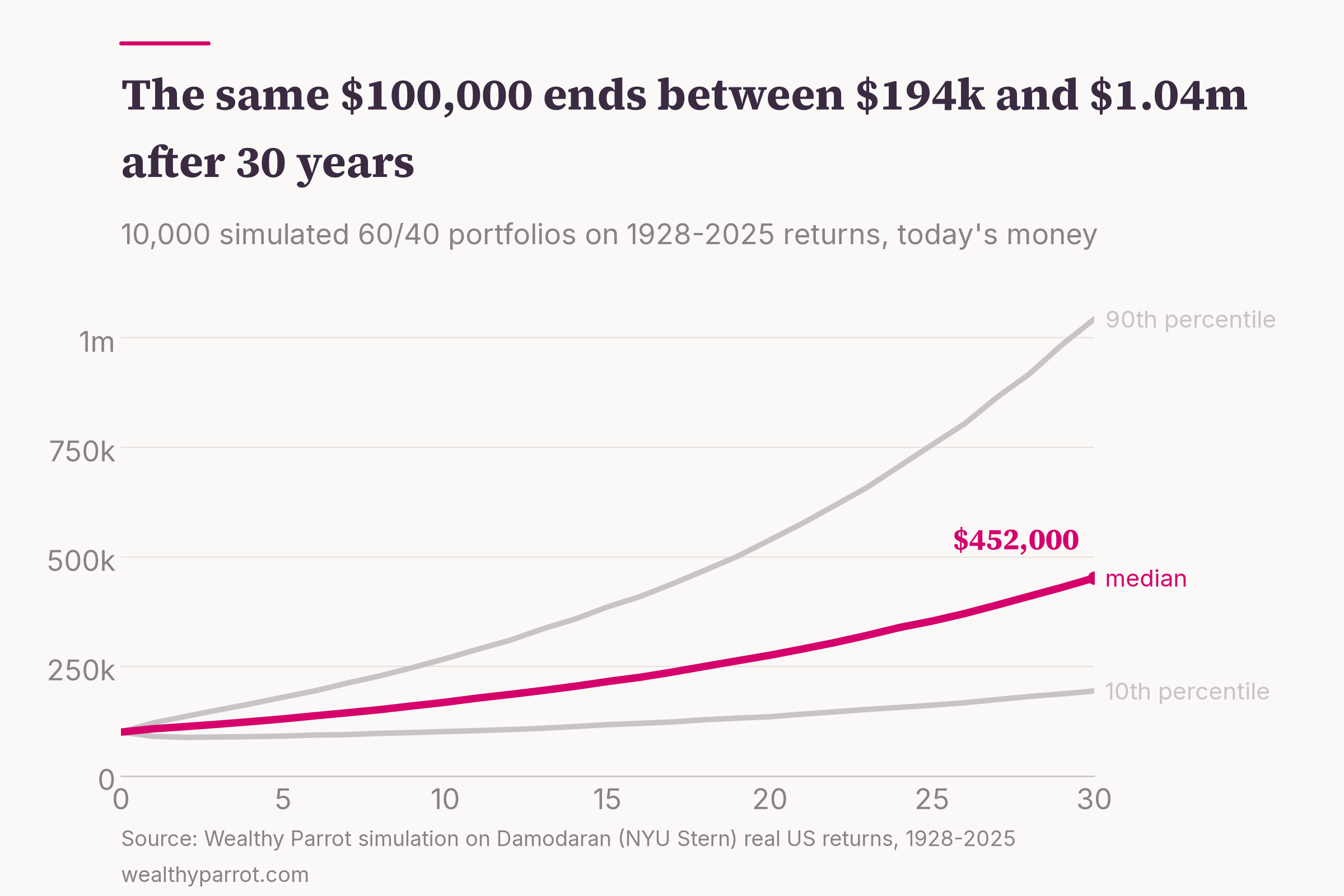
The median run ended at $452,000. One run in ten ended below $194,000, and one in ten above $1.04 million. The unluckiest of the 10,000 finished at $30,000 and the luckiest at $3.77 million, from the same portfolio and the same history.
The median is lower than the average return would suggest, and that's normal. A 5.9% average return with big swings compounds at only about 5.1% a year, and $100,000 growing at 5.1% for 30 years comes to roughly $450,000 (yes, almost exactly the median). Volatility eats into growth, which is the same arithmetic as the 20%-up, 20%-down example earlier.
The other thing the chart shows is how wide the range gets with time. After 10 years, the 10th percentile was $101,300, barely above the starting $100,000. So in one run in ten, a decade of patience had earned almost nothing after inflation, or had lost money. Over 30 years, just 1.2% of runs ended below where they started.
Monte Carlo vs history: testing a 4% withdrawal
Most people meet Monte Carlo in retirement planning, as a "probability of success." So I ran the classic test. Start with $1 million in the same 60/40 portfolio and take out $40,000 in the first year (4%). Raise it with inflation every year after that, and count how often the money runs out within 30 years.
I tested it three ways on the same 98 years of data. The historical method plays out every real 30-year period, starting in 1928, 1929 and so on up to 1996, which gives 69 retirements. The Monte Carlo reshuffle draws random years, as above. The Monte Carlo bell curve draws from a normal distribution with the same average, volatility and stock-bond correlation as the real data.
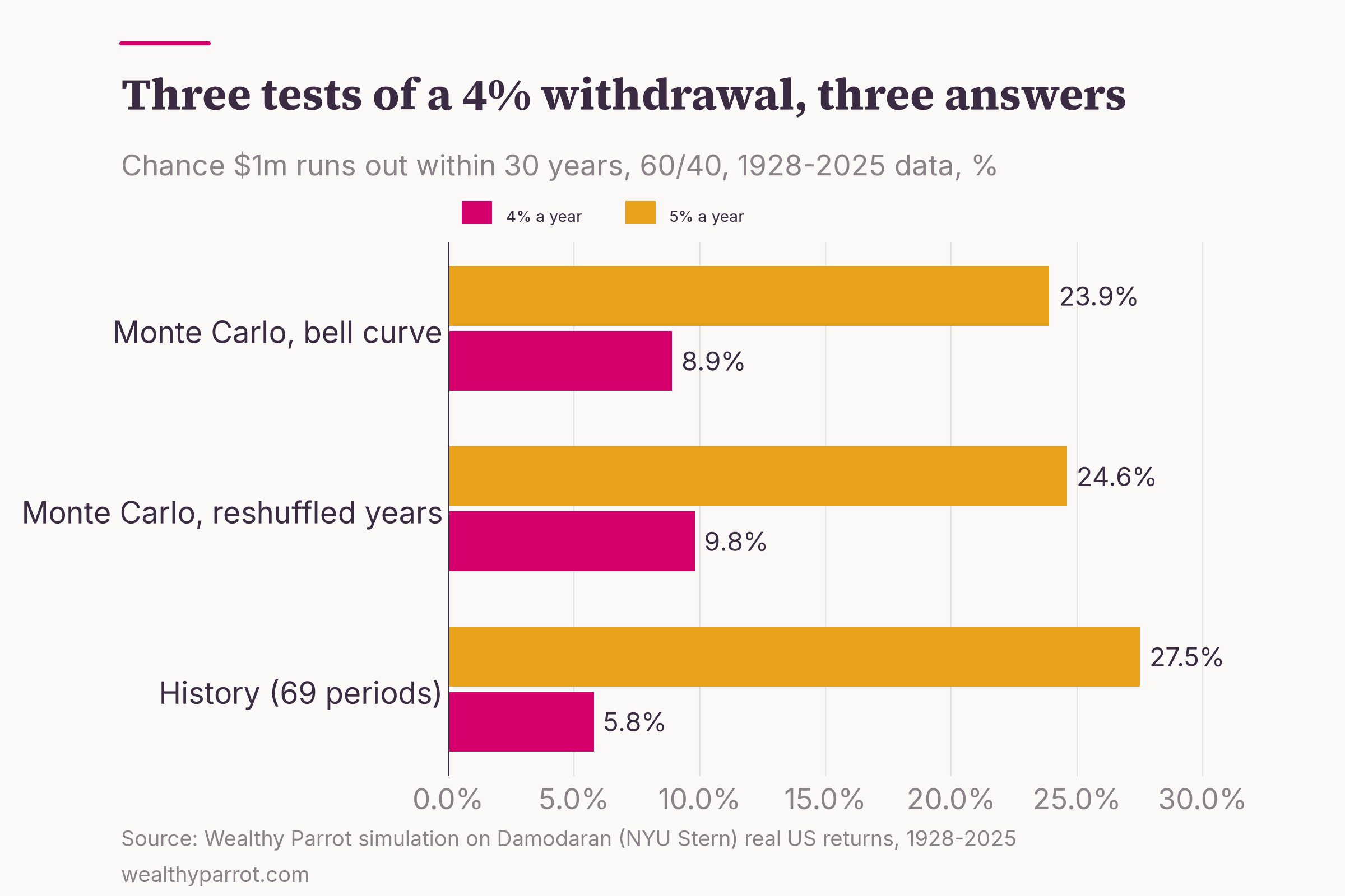
At 4%, the money ran out in 4 of the 69 historical retirements (5.8%), all of which started between 1965 and 1969, just before a decade of high inflation and weak markets. The reshuffled simulation failed 9.8% of the time and the bell curve 8.9%. At 5% a year, the three methods agreed more closely, at 27.5%, 24.6% and 23.9%.
Why does Monte Carlo look gloomier at 4%? History has only 69 retirements, and they overlap heavily, since the 1965 and 1966 retirees lived through 29 of the same years. Depending on how you count, that's barely three truly separate 30-year periods. Monte Carlo builds sequences that never happened, including some worse than anything in the record, so it finds failures that history simply didn't have time to produce.
That's also why the person who made the 4% rule famous still prefers history. In A Richer Retirement, the financial planner William Bengen reconstructs 388 retirees who retired at the start of every quarter from 1926 to 2022, using actual returns and inflation. He contrasts that approach with the random simulations other researchers use. In his data, the worst case still allowed a starting withdrawal of 4.7%.
Fun fact: Bengen's single worst retiree, the one who sets his famous safe rate, retired on 31 October 1968. Every other start date in his data could have taken out more.
What the professionals do with it
Big research shops run the same kind of exercise every year, with forecasts in place of history. Morningstar's 2025 retirement income research put the highest safe starting withdrawal rate at 3.9% for retirees who want a fixed, inflation-adjusted income, assuming a 90% probability of having money left after 30 years. It uses forward-looking return and inflation assumptions rather than history.
That number moves around with markets. Morningstar's base case was 3.3% in 2021, 3.8% in 2022, 4.0% in 2023 and 3.7% last year, mostly because bond yields and stock valuations changed. The method stayed the same and the inputs didn't.
The inputs can move the answer much further than that. In The Missing Billionaires, the investors Victor Haghani and James White ran a Monte Carlo on a portfolio of 60% stocks and 40% cash-like Treasury bills. With their assumptions, a 4% withdrawal ran out about one time in three over 30 years, and a 5% withdrawal about two times in three. Same rule, same method, very different inputs, and an answer roughly three times worse than my historical reshuffle.
Where Monte Carlo misleads
Monte Carlo is a good tool used badly more often than not. Here are the four traps I'd watch for, whichever tool you use.
Your inputs are the answer
The simulation can't know anything you didn't tell it. To show how sensitive it is, I re-ran the 4% retirement test with every year's return cut by 2 percentage points. The failure rate went from 9.8% to 27.0%.
So when a tool shows you "92% probability of success," ask yourself one thing first. Do you know what returns it assumed? If it used the last century of US returns, as my run did, you're assuming the next 30 years will look like that century.
Bell curves and correlations
Real returns have fatter tails than a bell curve. On yearly data, though, the difference was small in my run (8.9% failure with the bell curve versus 9.8% reshuffling real years). The bigger trap is assuming stocks and bonds always offset each other.
Fun fact: In real terms, 2022 was the second-worst year for a 60/40 portfolio in the whole 1928-2025 record, at -22.9%, worse than 2008 (-13.9%) or 1931 (-19.9%). Stocks lost 23.0% after inflation and bonds 22.8%, so the cushion vanished.
"90% success" is often too confident
The financial planning researchers Derek Tharp and Justin Fitzpatrick checked how well different Monte Carlo models would have predicted real outcomes. Their 2023 study on Kitces.com made forecasts at every point from 1951 to 2002. The traditional bell-curve model was overconfident above 50%. Of 100 clients aiming for a 95% chance of success, you'd expect 5 to fall short, and in their test 20 would have found they were spending too much.
Models built on historical data, or on market regimes, did better, with forecast errors about 25% lower than the traditional model. The authors note that the weaker methods are the ones most commonly used.
Fun fact: The study borrows a term from weather forecasting. A forecast that underpredicts rain has a "dry bias," and TV forecasters often lean the other way on purpose, because viewers mind a surprise downpour far more than an umbrella they didn't need.
Failure isn't a cliff
A simulation usually counts "success" as never running out, with fixed spending no matter what happens. Real people don't behave like that. If markets fall early in retirement, most retirees cut back a little, and that alone changes the odds a lot (I covered the practical versions in how you actually withdraw the money).
The other side matters too. In my reshuffled run, the median 4% retiree finished the 30 years with $1.59 million after inflation, more than they started with, and 65% of runs ended above $1 million. That's its own kind of failure if you spent 30 years being careful for nothing. Morningstar's own summary of its research makes the same point, that retirees "can increase their spending power by taking a more flexible approach."
Free Monte Carlo tools
You don't need to write code to run one, and the free options are good. What matters is knowing which return model each one uses.
Portfolio Visualizer has a free plan for personal use with no login required. Its Monte Carlo page offers four ways to generate returns. You can draw historical years at random (one at a time or in blocks), enter your own forecast, use the average, volatility and correlations of your assets, or pick a statistical distribution.
You can add contributions and several kinds of withdrawals. The block option is worth using, because it keeps runs of bad years together.
If you're comfortable with Python, okama is an open-source library (MIT licence) that runs Monte Carlo forecasts for portfolios with normal, lognormal or Student's t distributions, including withdrawals and contributions. You can fix the random seed, so a run is reproducible, which is how I'd recommend checking anyone's numbers, mine included.
A spreadsheet works too. In Excel or Google Sheets, the formula NORM.INV(RAND(), average, volatility) draws a random yearly return from a bell curve. Fill a row with 30 of them, compound them, copy the row 1,000 times and look at the percentiles. It's slow and blunt, and it teaches you more about the method than any website will.
For the question "when can I stop working?", my FIRE calculator is a simpler starting point, and you can then stress-test the answer with one of the tools above.
Practical takeaways
- Treat a Monte Carlo result as a range with odds, never a forecast. The useful number is usually the 10th percentile, not the median.
- Before you trust a "probability of success," find out what returns the tool assumed. Cutting returns by 2 points nearly tripled the failure rate in my test.
- Check a result with two methods, such as reshuffled history and a cautious forecast. If they disagree a lot, the assumptions are doing the work.
- Don't read 90% or 95% literally. In the Kitces test, 95% plans fell short four times as often as they promised.
- Plan for flexibility. A rule to trim spending after a bad year does more for your odds than an extra decimal place of simulation accuracy.
Ulam's real insight in 1946 wasn't about solitaire. It was that when a problem is too messy to solve, you can learn a lot by playing it out many times and counting. That works for your portfolio as well as it worked for neutrons, as long as you remember that the cards you deal are the assumptions you chose.